How to Calculate Sample Size for a Dissertation: Formulas, Power Analysis and Worked Examples

How to calculate sample size for a dissertation starts with one question: are you estimating something, such as a percentage or an average, or testing something, such as a difference between groups or a relationship between variables? Estimating points you to a precision formula like Cochran’s. Testing points you to a power analysis. Interviews follow a different logic altogether.

Before you pick a method, it helps to settle four questions:

• How many participants do I need, and who counts towards that number?
• Should I use a formula, a table or a power analysis?
• What do I do if I can only reach 40 people?
• How do I write the justification so my marker accepts it?

The worked examples cover quantitative designs first (surveys, group comparisons, correlation, regression), then interviews and focus groups. If you want to test your own numbers as you read, the free dissertation sample size calculator works alongside this guide.

What is the right sample size for a dissertation?

There is no single right number. The right sample is the smallest one that answers your research question with a precision or power you can defend, given the people you can realistically reach.

Two approaches cover most quantitative dissertations. A precision-based calculation asks how narrow you want your confidence interval to be. A power-based calculation asks how small a difference you need to detect, and with what certainty. Rosie Cornish’s Statstutor handout makes the same split, and adds a warning worth remembering: time, cost and availability of participants often limit a study, but they should not decide the number on their own, because a study that is too small simply produces inconclusive results.

Southampton’s library guide adds a timing rule. Sample size calculations should happen before you collect data, not after.

Which sample size method fits your dissertation?

Match your design to the method first. The wrong method gives a precise-looking number that answers the wrong question.

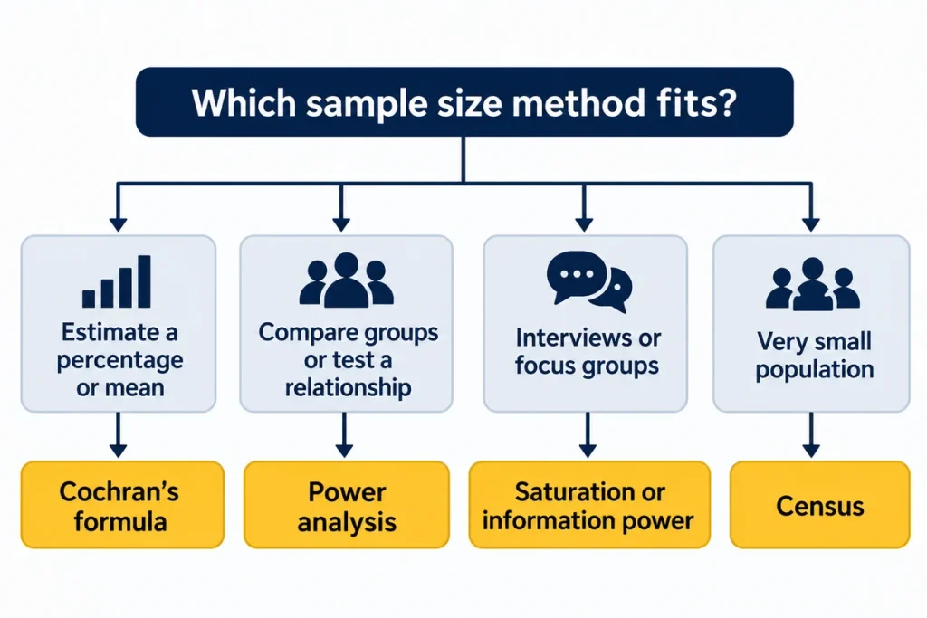
Your dissertation is…	Use	You need to know
Surveying to estimate a percentage	Cochran’s formula	Confidence level, margin of error, expected proportion, population size if known
Surveying to estimate an average	Precision formula for a mean	Standard deviation (from earlier studies or a pilot), margin of error
Comparing groups or testing a relationship	Power analysis	Effect size, significance level, power, the statistical test
Running a regression with several predictors	Power analysis for that model	Effect size, number of predictors; rules of thumb only as a check
Interviewing or running focus groups	Saturation or information power	Aim, how specific the sample is, how rich the data are
Studying a very small population	Census, then no sampling	The full list of eligible people
Using a dataset someone else collected	Sensitivity analysis	The N you have, significance level, power

Terms you need before using any sample size formula

• Confidence level: how sure you want to be that your interval captures the true value. 95% is the usual choice, with a Z-score of 1.96.
• Margin of error: the plus or minus around your result. A smaller margin needs a bigger sample.
• Population size: everyone who meets your eligibility criteria, such as all 1,200 final-year students in a faculty.
• Effect size: how big a difference or relationship you expect, or the smallest one worth detecting.
• Significance level (alpha): your cut-off for calling a result significant, usually 0.05.
• Power: the probability of detecting a real effect. It equals 1 minus beta, where beta is the chance of a Type II error. Targets of 0.80 or 0.90 are common.
• Response rate: the share of invited people who complete your survey. It decides how many invitations you send.

Sample size formula for surveys: Cochran’s formula step by step

Use Cochran’s formula when your survey estimates a percentage, such as the share of nursing students who report burnout. The formula is:

n0 = Z² × p × (1 – p) ÷ e²

Here Z is the Z-score for your confidence level, p is the expected proportion, and e is the margin of error written as a decimal. If you have no prior estimate of p, use 0.5, which gives the largest and safest sample. For 95% confidence and a 5% margin of error:

1.96² × 0.5 × 0.5 ÷ 0.05² = 384.16, which you round up to 385. Always round up, never down. Some calculators show 384, but 385 is the safe minimum.

Cochran’s formula for a smaller, known population

When you know the population and it is not huge, apply the finite population correction:

n = n0 ÷ (1 + (n0 – 1) ÷ N)

Take a faculty of 1,200 students. With n0 = 385, the corrected sample is 385 ÷ (1 + 384 ÷ 1,200) = 291.7, so you need 292 completed responses. Population size matters most for small groups. Krejcie and Morgan’s 1970 table, which many dissertations cite, shows the same pattern at 95% confidence and a 5% margin: 80 for a population of 100, 278 for 1,000, and 384 for 1,000,000.

How confidence level and margin of error change the number

These figures assume p = 0.5 and a very large population. They show how quickly a tighter margin raises the cost.

Confidence level	10% margin	5% margin	3% margin
90%	68	271	752
95%	97	385	1,068
99%	166	664	1,844

Halving the margin of error multiplies the sample by four. Moving from a 5% to a 2.5% margin at 95% confidence takes you from 385 to 1,537. Statstutor states the general rule: to improve precision by a factor of k, you need k² times as many participants.

Yamane’s formula and when it misleads

Yamane’s formula (often called Slovin’s formula) is n = N ÷ (1 + N × e²). For 1,200 students and a 5% margin it gives 1,200 ÷ (1 + 1,200 × 0.0025) = 300, close to Cochran’s 292.

Be careful with it. It builds in a 95% confidence level and p = 0.5, so it only suits estimating a proportion. Statisticians also criticise it for being applied to problems it was never built for, such as estimating means. If your supervisor asks for a confidence level other than 95%, or you expect a proportion far from 0.5, use Cochran’s formula instead.

Sample size formula for estimating an average

For a mean, rearrange the confidence interval so that n = (Z × s ÷ E)², where s is the standard deviation and E is the margin you can tolerate in the units of your scale. Suppose earlier studies report a standard deviation of 4 points on a stress scale and you want to be within 1 point at 95% confidence. Then n = (1.96 × 4 ÷ 1)² = 61.5, so you need 62 responses. The standard deviation is an assumption, so say where it came from.

How to calculate sample size with power analysis

Use a power analysis when you test a hypothesis: two groups differ, two variables correlate, or a predictor explains an outcome. You give the calculation four things, and it returns the fifth: effect size, significance level, power, the statistical test, and the required sample size.

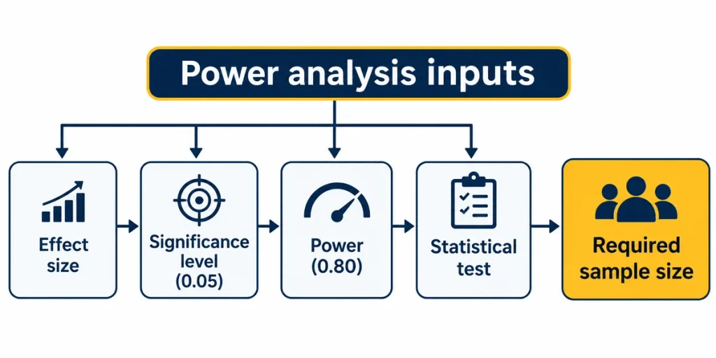
The test matters because each one has its own formula. Settle your hypotheses first, then use the statistical test selector to name the test you will actually run. A sample size calculated for a simple correlation does not automatically cover a regression with six predictors.

Choosing an effect size you can defend

The effect size is the input students find hardest, and it has the biggest influence on the answer. You have three honest sources. First, similar published studies in your field. Second, a small pilot. Third, the smallest difference that would matter in practice, which Statstutor recommends deciding before you start.

Cohen’s conventional benchmarks (d = 0.2, 0.5 and 0.8 for small, medium and large differences between two means) are a fallback, not a justification. They are rough heuristics, and the right effect depends on your discipline. The size of the difference you want to detect changes everything. In Statstutor’s heart attack example, detecting a fall in deaths from 10% to 5% needs 578 patients per group at 90% power. Detecting a fall from 10% to 8% needs 4,295 per group.

Sample sizes at 80% power for common tests

The table below uses a two-sided significance level of 0.05 and 80% power. Use it to sense-check your own calculation, not to replace it.

Analysis	Effect size	Sample needed
Independent-samples t-test	Small (d = 0.2)	About 394 per group
Independent-samples t-test	Medium (d = 0.5)	About 64 per group (128 in total)
Independent-samples t-test	Large (d = 0.8)	About 26 per group (52 in total)
Paired-samples t-test	Medium (d = 0.5)	About 34 pairs
Pearson correlation	r = 0.3	About 85
Pearson correlation	r = 0.5	About 30
One-way ANOVA, three groups	Medium (f = 0.25)	About 53 per group (159 in total)

Software can differ from these figures by a participant or two, depending on the method it uses. Aiming for 90% power raises the independent t-test example (d = 0.5) from 64 to 86 per group. Statstutor’s table-based method gives 84 for the same inputs, because it uses an approximation. Report the figure your software gives, and name the software.

One practical point on the large-effect row. Only plan around d = 0.8 if earlier studies in your field really report effects that big. A small sample built on an optimistic effect size is the most common way to end up underpowered.

How to run a sample size calculation in G*Power, SPSS or R

G*Power is the tool most dissertation supervisors expect. The team at Heinrich Heine University Düsseldorf publishes it free for everyone, and it covers t tests, F tests, chi-square tests, z tests and some exact tests. It also draws graphs of power against sample size. Windows version 3.1.9.7 and Mac version 3.1.9.6 are listed on the official G*Power download and reference page, which also gives the two papers to cite (Faul et al., 2007 and 2009). Position correct as of November 2026; check the download page for the current version.

Here is the routine for a paired-samples t-test, which follows the pattern Southampton’s library guide sets out:

1. Choose “t tests” in the Test Family menu.
2. Choose “Means: Difference between two dependent means (matched pairs)” as the statistical test.
3. Choose “A priori: Compute required sample size” as the type of power analysis.
4. Enter your effect size, an alpha of 0.05 and a power of 0.80 or 0.90.
5. Click Calculate, then save a screenshot of the inputs and output for your appendix. The G*Power terms of use allow screenshots without asking permission.

For an independent-samples t-test with d = 0.5, alpha 0.05 and power 0.80, you should see 64 per group, 128 in total. Other tests follow the same steps with different effect size inputs: Cohen’s d for t tests, f for ANOVA, f² for regression.

SPSS offers a Power Analysis option under the Analyze menu, and R users can use the pwr package, for example pwr.t.test for t tests and pwr.r.test for correlations. Whichever you use, leave the sample size field blank so the program solves for it.

What if you cannot reach the required sample size?

This happens to many students, and the answer is not to hide it. Run a sensitivity analysis instead. G*Power supports this alongside the a priori analysis: you enter the sample you can realistically get, plus alpha and power, and it tells you the smallest effect you can reliably detect.

For an independent t-test at 80% power and alpha 0.05, 40 per group can only detect an effect of about d = 0.63, and 25 per group needs about d = 0.81. Say that plainly in your methodology and limitations: your study can detect medium-to-large effects, and a non-significant result for a smaller effect is inconclusive, not evidence of no effect.

Two design choices can help. A paired design often needs fewer participants, because differences within the same person vary less than differences between people (this is a standard feature of paired designs). Discuss either option with your supervisor before collecting data.

Sample size for regression, ANOVA and correlation dissertations

Regression is where rules of thumb cause trouble. Samuel Green’s 1991 study compared several of them against power analysis. It found support for N of at least 50 + 8m to test the overall model, and at least 104 + m to test individual predictors, where m is the number of predictors. With five predictors that means 90 and 109 respectively.

Treat these as a quick check only. They assume a medium-sized relationship, and later work by Scott Maxwell found that historical rules of thumb are often inaccurate for individual predictors. If your expected effect is small, or you have interaction terms, run a proper power analysis for the model you will report. For ANOVA and correlation, the table above gives the reference points.

Allow for dropout and low response rates

Every calculation above gives the number you need to analyse. You must recruit more. Statstutor lists the usual causes: non-response, withdrawal, people lost to follow-up, and missing answers.

Use this adjustment: recruitment target = required sample ÷ (1 – expected loss rate). If power analysis says you need 128 and you expect to lose 20%, recruit 128 ÷ 0.80 = 160.

Surveys need a second step. If you need 292 completed responses and past surveys in your setting got around a 30% response rate (an assumption you must source yourself), you must invite about 292 ÷ 0.30 = 974 people. Plan the invitation route when you design your survey questionnaire, not afterwards.

Sample size for interviews and focus groups

Qualitative dissertations do not use power analysis, because you are not testing a hypothesis or estimating a population value. Instead, your sample is adequate when it gives you rich enough data to answer the question. Three sources help you defend a number.

• Guest, Bunce and Johnson (2006) found that most codes in a fairly uniform group of interviewees had appeared by the twelfth interview, with the basic elements of the main themes visible as early as six.
• Hennink and Kaiser (2022) reviewed 23 studies of saturation. Studies with empirical data reached it within 9 to 17 interviews or 4 to 8 focus group discussions, especially where the population was homogeneous and the objectives narrow. Multi-country studies and studies chasing deeper “meaning” saturation needed larger samples.
• Malterud, Siersma and Guassora (2016) proposed “information power”: the more relevant information your sample holds, the fewer participants you need. They link it to five things: the aim of the study, how specific the sample is, use of established theory, quality of dialogue, and analysis strategy.

Treat these ranges as evidence for your justification, not as a fixed minimum. Saturation depends on your design, so explain how you judged it. For example, report that no new codes appeared in the last few interviews you analysed. The guide to semi-structured interviews covers recruitment and topic guides, and the walkthrough of thematic analysis shows how to track codes as you go.

Small populations, secondary data and case studies

Sometimes the sensible answer is no sample at all. If your population is small, such as 60 staff in one department, a census of everyone eligible removes sampling error. SmartSurvey makes the same point for groups of around 100.

With secondary data, the dataset fixes your N. Use a sensitivity analysis to state which effects that N can detect, and describe the dataset’s own sampling design. In a case study, the number of cases is justified by case selection logic, not by a formula, so explain why each case was chosen.

How to justify your sample size in the methodology chapter

Markers look for the reasoning behind the number, not just the number. A complete justification covers these points:

• The target population and who was eligible.
• The sampling strategy and why it suits your question.
• The planned primary analysis, since the calculation must match it.
• Every input: effect size and its source, alpha, power or confidence level, margin of error.
• The formula or software used, with its citation.
• The adjustment for dropout or non-response.
• Honest limits, including what your final sample can and cannot detect.

Here is an example for an experiment. Square brackets mark the parts you must replace with your own sources and values:

An a priori power analysis was run in G*Power 3.1 (Faul et al., 2007) for an independent-samples t-test. Assuming a medium effect (d = 0.5, based on [cite the study you used]), a two-tailed alpha of 0.05 and power of 0.80, the minimum sample was 64 participants per group (128 in total). Allowing for 20% attrition, the recruitment target was 160 participants.

And here is one for a survey:

The population comprised [1,200] students. Using Cochran’s formula with a finite population correction (Cochran, 1977), 95% confidence, a 5% margin of error and an expected proportion of 0.5, the minimum sample was 292 completed responses. Assuming a response rate of [30%, source], [974] students were invited.

Cite the original textbook or paper you actually read, not a calculator website. Place the justification in your methodology chapter, and make sure the number matches your ethics approval application, since both documents should state the same target.

Common sample size mistakes to avoid

• Copying a number from another dissertation. “Previous studies used 30” is not a justification unless those studies share your design, population and analysis.
• Using Yamane or Slovin for everything. It only fits estimating a proportion at 95% confidence.
• Rounding down. Always round up to the next whole participant.
• Choosing an effect size from nowhere. Cite a source or state the smallest difference that matters.
• Calculating for the wrong test. Base the number on your primary analysis, or on whichever planned test needs the most participants.
• Forgetting dropout. The analysable sample and the recruited sample are different numbers.
• Running power after the fact. Power belongs to the planning stage. Explain a non-significant finding in your results chapter through effect sizes and confidence intervals instead.

Sample size questions students ask

Is 30 participants enough for a dissertation?

Only if your analysis supports it. A medium effect in two independent groups needs about 64 per group at 80% power. Thirty in total can detect only very large effects.

Does population size change the sample size?

For small populations, yes. For large ones, hardly at all. At 95% confidence and a 5% margin, the Krejcie and Morgan table moves from 370 for a population of 10,000 to 384 for 1,000,000.

Do I need a power analysis for a survey?

Only if you test hypotheses with it, such as comparing groups or correlating variables. A descriptive survey that estimates percentages needs a precision calculation like Cochran’s. Many surveys do both, so base the number on whichever requirement is larger.

Can I use an online calculator?

Yes, if you understand its inputs and report them. Check that the calculator matches your design. A proportion calculator cannot size an ANOVA.

Next steps once you have your number

Write the justification while the calculation is fresh, and keep your G*Power screenshot or calculation notes. Then confirm the analysis itself with the guide to choosing a statistical test, so the test, the sample and the research question all line up.

If you want a second pair of eyes on the wording of your sampling section, dissertation methodology support can review the reasoning with you. Use any model or reference work as learning material and follow your own university’s academic integrity policy.