
How to Clean and Analyse Survey Data in SPSS: A Step-by-Step Workflow for Your Dissertation

I have 200 questionnaire responses in an Excel file. How do I clean survey data in SPSS before I run anything? What happens to blank answers, double submissions and the respondent who typed an age of 190? Once the file is clean, how do I analyse Likert scale items without my supervisor sending the results chapter back?
Clean first, analyse second, and write down every change you make. For most undergraduate and Master’s questionnaires the order is: import, label, screen for impossible values, declare missing codes, remove duplicates, flag careless answers, check outliers, reverse-code, build scale scores, then describe and test. Every stage below comes with the SPSS menu route and the decision you will need to defend in your methodology chapter. The steps are for SPSS, and menu wording can differ slightly between versions.
How to clean and analyse survey data in SPSS: the workflow at a glance
Each stage leaves a trace you can put in a cleaning log. That log is what turns “I tidied the data” into evidence an examiner can check.
| Stage | SPSS route | What to record |
|---|---|---|
| 1. Import and save | File, Open, Data | Source file name and number of cases imported |
| 2. Set up variables | Variable View: Name, Label, Values, Missing, Measure | Your codebook |
| 3. Screen values | Analyze, Descriptive Statistics, Frequencies | Out-of-range values and what you did |
| 4. Declare missing codes | Variable View, Missing column | Codes defined and counts per item |
| 5. Remove duplicates | Data, Identify Duplicate Cases | Matching rule and cases removed |
| 6. Flag careless answers | Transform, Compute Variable | Cases flagged and cases removed |
| 7. Check outliers | Analyze, Descriptive Statistics, Explore | Values checked and the decision |
| 8. Reverse-code | Transform, Recode into Different Variables | Items reversed |
| 9. Scale scores and reliability | Transform, Compute Variable; Analyze, Scale, Reliability Analysis | Items per scale, missing-item rule, alpha |
| 10. Describe and test | Frequencies, Descriptives, then your chosen test | Final number of cases for each analysis |
Protect your raw data and start a cleaning log
Keep the original export untouched in its own folder and do all cleaning on a copy. Save each stage as a new file, such as survey_01_imported.sav and survey_02_cleaned.sav, so you can step back if a decision proves wrong.
Open a simple table with five columns: issue, how you found it, action taken, reason and date. A line such as “Respondent 87 reported age 190; impossible; set to missing; no way to verify” is enough. Store the files where your ethics approval says survey data must be kept, and remove direct identifiers such as names or emails from the working file if your approval requires it.
How to import survey data into SPSS from Excel or CSV
Prepare the spreadsheet first: one header row, one respondent per row, short variable names without spaces, and no totals rows or merged cells. If your survey tool can export a .sav file directly, as Qualtrics can (UNSW Sydney, n.d.), you can skip Excel altogether, but check which labels came across.
- Choose File, then Open, then Data. Change the file type from .sav to Excel and select your file (La Trobe University Library, n.d.).
- Tick “Read variable names from the first row of data”. If you leave it unticked, SPSS treats the header row as a respondent (UCLA OARC, n.d.).
- Pick the worksheet that holds the responses. SPSS imports one sheet at a time (Saarland University, n.d.).
- Save immediately as a .sav file, then compare the number of rows in SPSS with the number in Excel. A mismatch now is far cheaper to fix than one found in the results chapter.
Set up variable names, labels and measurement levels in Variable View
Switch to Variable View and work through the columns. Name each variable briefly (q1, q2, age). Use Label for the full question wording. Use Values to attach the answer labels, for example 1 = Strongly disagree through 5 = Strongly agree. Use Missing for non-answer codes, covered in the next section. Use Measure to declare each variable as nominal, ordinal or scale (Bates College Libraries, n.d.).
For a typical student wellbeing questionnaire, Likert items are usually ordinal, gender and course are nominal, and age or hours of study are scale. Keep items of the same scale next to each other in the file, because the shorthand q1 TO q10 in SPSS syntax follows file order. Your codebook is simply this Variable View information saved in a table. If you are still drafting items, building a dissertation questionnaire explains how wording and coding choices affect analysis later.
Screen survey data for impossible and out-of-range values
Run frequencies on every variable before anything else. Choose Analyze, then Descriptive Statistics, then Frequencies, move all items across and read the minimum and maximum. A 1 to 5 item showing a 7, a 0 or a stray 55 is a data-entry or export fault.
FREQUENCIES VARIABLES=q1 TO q10 age.Find the offending case, return to the raw export and correct the value only if the source proves what it should be. If nothing can verify it, set it to missing and log the decision. Guessing what the respondent “probably meant” is the one fix an examiner cannot accept.
How to handle missing values in SPSS
SPSS recognises two kinds of missing value. System-missing means a numeric cell is empty and shows as a full stop in Data View. User-missing means a real number you have declared as a non-answer, such as 99 for “prefer not to say” (UCLA OARC, n.d.).
This distinction matters because an undeclared 99 is just a very large answer, and it will drag your means upwards. IBM’s own example is a questionnaire item where “Don’t know” is coded 5: if you want it treated as missing, it must be declared user-missing (IBM, n.d.a). To declare codes, click the Missing cell for the variable in Variable View. You can define up to three separate values, or a range plus one extra value (IBM, n.d.b). Text variables behave differently: blanks count as valid unless you define a single space as missing (IBM, n.d.b).
MISSING VALUES q1 TO q10 (99).
FREQUENCIES VARIABLES=q1 TO q10.
Check the frequency tables afterwards: the declared code should now sit under Missing, not Valid. By default, SPSS treats user-missing values the same way as system-missing ones in analyses (IBM, n.d.e).
What to do with missing answers in a dissertation survey
Do not replace blanks with zero, and do not delete a respondent just because one answer is absent. Start by looking for a pattern. If one question has far more blanks than the rest, the wording or routing may be the cause, and that belongs in your limitations.
Then accept that SPSS handles missing data differently from one procedure to the next. Descriptives uses whatever valid values exist for each variable, correlations default to pairwise deletion, and Reliability Analysis offers only listwise exclusion (UCLA OARC, n.d.; SPSS Tutorials, n.d.a). So your number of cases will change between analyses, and each table should state its N. Statistical imputation exists, but SPSS provides it through a separate Missing Values option or the Professional edition (IBM, n.d.c), so agree with your supervisor before using it. Leaving missing answers as missing and reporting the N is a defensible default for a small project.
Find and remove duplicate survey responses in SPSS
Duplicates arise from data-entry errors, respondents submitting twice, or export problems (IBM, n.d.d). To flag them, choose Data, then Identify Duplicate Cases. Move one or more variables that define a match into the matching box, such as a respondent ID, or a combination of start time and demographics if there is no ID. Tick the option that creates a variable marking primary and duplicate cases, and tick the option to move matching cases to the top so you can inspect them. IBM’s documentation on identifying duplicate cases lists these options in full.
Treat the output as a list to examine, not a delete command. IBM Support has documented a case where the tool missed a duplicate held in a text identifier (IBM Support, n.d.), so cross-check with Frequencies on the ID variable. Decide your rule before deleting anything, for example “keep the first complete submission”, and write it in the log along with the number of cases removed. Filtering hides cases, while Select Cases with “Delete unselected cases” removes them for good (IBM, n.d.d), so keep a copy of the file from before deletion.
Flag straight-lining and other careless responses
Some respondents click the same option all the way down the page. Spotting them is easy with the within-case standard deviation, which is zero when every answer is identical (SPSS Tutorials, n.d.b). Compute it across the items of one block, including negatively worded ones, because identical answers to opposite statements suggest the person was not reading.
COMPUTE row_sd = SD(q1 TO q10).
EXECUTE.
FREQUENCIES VARIABLES=row_sd /FORMAT=NOTABLE /STATISTICS=MINIMUM.
A zero is a flag, not proof. On a short block, someone can honestly answer “agree” five times running. Read the flagged cases alongside completion time if your survey tool exports it, and state in your methodology how you decided who to exclude. Do the same for any exclusion rule you applied to the whole sample, such as respondents who did not meet the eligibility criteria.
How to detect outliers in SPSS (and when to keep them)
Outliers matter for continuous variables such as age, hours worked or spending, and for scale scores. A single Likert item bounded between 1 and 5 cannot have an impossible outlier, so there is nothing to detect there beyond the screening you have already done.
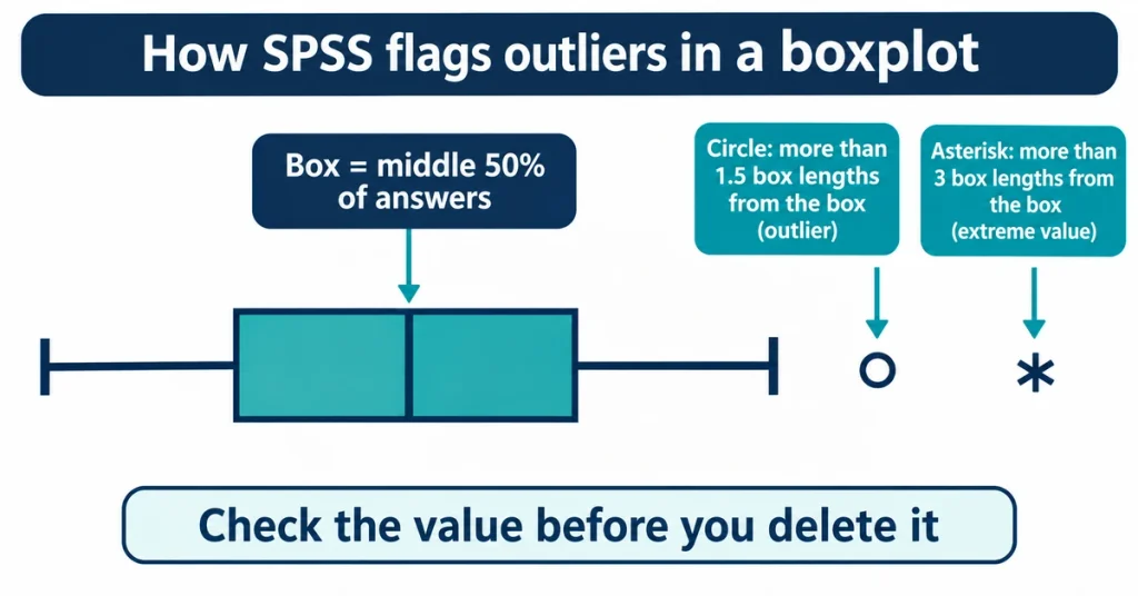
Choose Analyze, then Descriptive Statistics, then Explore. Put the variable under Dependent List, request boxplots and tick Outliers under Statistics to get the Extreme Values table.
EXAMINE VARIABLES=hours_study
  /PLOT BOXPLOT
  /STATISTICS EXTREME.
SPSS boxplots mark a value with a circle when it sits more than 1.5 interquartile ranges beyond the box, and with an asterisk as an extreme value when it sits more than 3 beyond it (SPSS Tutorials, n.d.c). That is a rule of thumb, not a statistical law (Statistics How To, n.d.). So the flag starts an investigation, and the question is why the value exists.
- Typing or export error: correct it from the source, or set it to missing if you cannot verify it.
- Genuine but unusual answer: keep it. A student who really studies 60 hours a week is data, not noise.
- Unsure: run the analysis with and without the case and report both if the conclusion changes.
Reverse-code negatively worded items in SPSS
Suppose a belonging scale includes “I often feel isolated on campus” beside positively worded items. A high score on that item means low belonging, so it must be flipped before you total the scale. SPSS has no dedicated reverse-coding menu, so you use the general recode procedure (Laerd Statistics, n.d.).
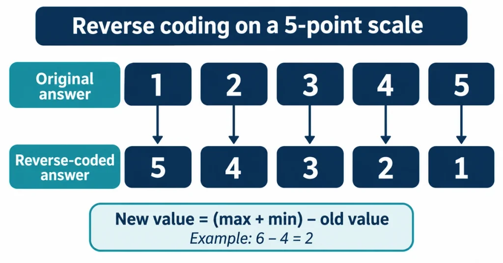
- Choose Transform, then Recode into Different Variables. This leaves the original untouched, whereas Recode into Same Variables overwrites it for good (Kent State University Libraries, n.d.a).
- Move the item across, type a new name such as q4_r and a label such as “q4 reverse coded”, then click Change.
- Click Old and New Values and add every pair: 1 to 5, 2 to 4, 3 to 3, 4 to 2, 5 to 1. Include the middle value even though it does not change, or SPSS can leave it empty in the new variable (SJU SPSS Guide, n.d.).
- Run frequencies on the old and new item. The counts should mirror each other.
RECODE q4 q7 (1=5) (2=4) (3=3) (4=2) (5=1) INTO q4_r q7_r.
EXECUTE.
On any scale, the reversed score equals the highest possible score plus the lowest, minus the original, so a 1 to 7 item becomes 8 minus the original. From now on, use q4_r in every scale calculation and leave q4 out.
Compute scale scores and test reliability with Cronbach’s alpha
Choose Transform, then Compute Variable, and build the score from the items of one scale. How you write the formula decides what happens to incomplete respondents. Adding items with plus signs makes the whole score missing if any single item is missing, whereas the MEAN function averages whatever is present (The Analysis Factor, n.d.). The suffix version, such as MEAN.3, only calculates a score when at least three items are valid (SPSS Tutorials, n.d.d).
COMPUTE belonging = MEAN.4(q1, q2, q3, q4_r, q5).
EXECUTE.
There is no universal cut-off for how many items a respondent may skip, so choose a rule (many researchers require most of the scale to be answered), justify it and apply it to every scale. Averaging only two of ten items can describe someone poorly.
Then test internal consistency with Analyze, then Scale, then Reliability Analysis, using the reversed items. A negative alpha almost always means a reversal was missed (SPSS Tutorials, n.d.e). The full walkthrough, including how to read item-total statistics and what values count as acceptable, is covered in checking reliability and validity.
How to analyse Likert scale data in SPSS
Start by deciding whether you are analysing single items or a combined scale, because the two are treated differently. Single Likert items are ordinal, so frequencies, percentages, the median and the mode describe them best. A scale built from several items is often analysed with means and standard deviations, and Sullivan and Artino (2013) report evidence that parametric tests tend to give sound answers with such data, although they note that a mean reported to many decimal places adds little.
Researchers still disagree on this, so state your position in the methodology chapter and cite a source for it. A short sentence such as “Individual items were summarised with medians and frequencies; the composite scale was treated as continuous” makes your reasoning visible.
FREQUENCIES VARIABLES=q1 q2 q3 q4_r q5
  /STATISTICS=MEDIAN MODE.
DESCRIPTIVES VARIABLES=belonging /STATISTICS=MEAN STDDEV MIN MAX.
For categorical survey data such as gender, year of study or yes/no answers, report counts and percentages from Frequencies. For continuous variables, Explore adds normality tests and Q-Q plots when you tick the normality option (Kent State University Libraries, n.d.b), which feeds the next decision.
Choose the statistical test that fits your research question
The test follows the research question, the variable types and the design, not the other way round. Comparing two groups on a scale score, relating two scores and predicting an outcome each call for different tests. Choosing a statistical test walks through the decision, and the statistical test selector narrows it from your data type.
If you want a second explanation of a specific SPSS procedure, the University of Sheffield’s SPSS guides cover tasks such as transferring data from Excel, recoding and checking normality.
How to report data cleaning in your dissertation
Put the rules in the methodology chapter and the numbers in the results. The methodology states how duplicates, missing answers, careless responses and outliers were identified and handled. The results open with a short account of how many responses arrived and how many remained. A cleaning log makes this section quick to write, and writing a dissertation results chapter shows where it fits.
Example wording, with placeholders for your own figures:
[Number] responses were received. [Number] duplicate submissions were removed, keeping the first complete response. [Number] cases were excluded for [stated reason]. Responses of [code] were treated as missing. Missing data were not imputed, and the number of cases is reported for each analysis. The final sample was N = [number].
Common mistakes when cleaning and analysing survey data in SPSS
- Cleaning the only copy of the data. Keep the raw export untouched.
- Leaving 99 or -9 undeclared, so it behaves like a real answer.
- Recoding into the same variable and losing the original answers.
- Running alpha on items before reversing the negative ones.
- Deleting every outlier automatically, including genuine answers.
- Forgetting that the number of cases differs between procedures, then reporting one N for everything.
- Choosing a test before the data have been cleaned and checked.
- Making cleaning decisions without a written rule, so they cannot be explained in the viva.
Survey data cleaning in SPSS: your questions answered
Can I clean the data in Excel and then import it into SPSS?
Yes, for formatting jobs such as removing header clutter, trimming spaces and fixing column names. Leave the judgement calls, such as missing codes, reverse coding and exclusions, to SPSS so they are recorded in syntax or the output you can save and show your supervisor.
How many missing answers are too many?
No single threshold applies to every survey. Set a rule before you look at the results, for example a minimum share of answered items per scale and for the whole questionnaire, justify it with a source or your supervisor’s advice, and apply it to every respondent.
Should I save my SPSS syntax?
Yes. Clicking Paste instead of OK in a dialogue box sends the command to a syntax file. Saving that file gives you a replayable record of the cleaning, which helps if a supervisor asks you to rerun something after a late response arrives.
Next step: turn the cleaned file into results
Finish the cleaning log, save the cleaned .sav file and write the methodology paragraph while the decisions are fresh. If the results chapter is where you are stuck, dissertation results help offers guidance on planning, structure and feedback on your own draft. Use any reference work according to your institution’s policy.
References for your methodology chapter
Bates College Libraries (n.d.) ‘SPSS: working with data’. Available at: https://libguides.bates.edu/spss/data (Accessed: 12 November 2026).
IBM (n.d.a) ‘IBM SPSS Missing Values’. Available at: https://www.ibm.com/docs/en/SSLVMB_31.0.0/pdf/IBM_SPSS_Missing_Values.pdf (Accessed: 12 November 2026).
IBM (n.d.b) ‘Missing values’, IBM SPSS Statistics documentation. Available at: https://www.ibm.com/support/knowledgecenter/SSLVMB_25.0.0/statistics_mainhelp_ddita/spss/base/idh_defvar_msval.html (Accessed: 12 November 2026).
IBM (n.d.c) ‘IBM SPSS Missing Values’ (Introduction to missing values). Available at: https://ibm.com/docs/SSLVMB_30.0.0/pdf/IBM_SPSS_Missing_Values.pdf (Accessed: 12 November 2026).
IBM (n.d.d) ‘Identifying duplicate cases’, IBM SPSS Statistics documentation. Available at: https://www.ibm.com/docs/SSLVMB_sub/statistics_mainhelp_ddita/spss/base/idh_idd_duplicatecases.html (Accessed: 12 November 2026).
IBM (n.d.e) ‘Overview (MISSING VALUES command)’, IBM SPSS Statistics documentation. Available at: https://www.ibm.com/docs/en/SSLVMB_23.0.0/spss/base/syn_missing_values_overview.html (Accessed: 12 November 2026).
IBM Support (n.d.) ‘SPSS Statistics: Identify Duplicate cases is not picking up a specific value’. Available at: https://www.ibm.com/support/pages/node/6405726 (Accessed: 12 November 2026).
Kent State University Libraries (n.d.a) ‘SPSS tutorials: recoding variables’. Available at: https://libguides.library.kent.edu/SPSS/RecodeVariables (Accessed: 12 November 2026).
Kent State University Libraries (n.d.b) ‘SPSS tutorials: descriptive stats for one numeric variable (Explore)’. Available at: https://libguides.library.kent.edu/SPSS/Explore (Accessed: 12 November 2026).
La Trobe University Library (n.d.) ‘IBM SPSS: data’. Available at: https://latrobe.libguides.com/ibmspss/data (Accessed: 12 November 2026).
Laerd Statistics (n.d.) ‘Reverse coding in SPSS Statistics’. Available at: https://statistics.laerd.com/spss-tutorials/reverse-coding-in-spss-statistics.php (Accessed: 12 November 2026).
Saarland University (n.d.) ‘SPSS introduction: data input and import’. Available at: https://moodle.uni-saarland.de/mod/resource/view.php?id=106324 (Accessed: 12 November 2026).
SPSS Tutorials (n.d.a) ‘Cronbach’s alpha in SPSS’. Available at: https://www.spss-tutorials.com/cronbachs-alpha-in-spss (Accessed: 12 November 2026).
SPSS Tutorials (n.d.b) ‘SPSS: quick overview statistical functions’. Available at: https://www.spss-tutorials.com/spss-main-statistical-functions/ (Accessed: 12 November 2026).
SPSS Tutorials (n.d.c) ‘Boxplots: what is it?’. Available at: https://www.spss-tutorials.com/boxplot-what-is-it/ (Accessed: 12 November 2026).
SPSS Tutorials (n.d.d) ‘How to compute means in SPSS’. Available at: https://www.spss-tutorials.com/how-to-compute-means-in-spss/ (Accessed: 12 November 2026).
SJU SPSS Guide (n.d.) ‘Recoding, computing variables, selecting cases, splitting files’. Available at: https://sites.google.com/sju.edu/spss-guide/recoding-computing-variables-selecting-cases-splitting-files (Accessed: 12 November 2026).
Statistics How To (n.d.) ‘Outliers in SPSS: overview’. Available at: https://statisticshowto.com/probability-and-statistics/outliers (Accessed: 12 November 2026).
Sullivan, G.M. and Artino, A.R. (2013) ‘Analyzing and interpreting data from Likert-type scales’, Journal of Graduate Medical Education, 5(4), pp. 541-542. Available at: https://pmc.ncbi.nlm.nih.gov/articles/PMC3886444 (Accessed: 12 November 2026).
The Analysis Factor (n.d.) ‘Averaging and adding variables with missing data in SPSS’. Available at: https://www.theanalysisfactor.com/averaging-and-adding-variables-with-missing-data-in-spss-2/ (Accessed: 12 November 2026).
UCLA OARC (n.d.) ‘Missing data in SPSS’. Available at: https://stats.oarc.ucla.edu/spss/modules/missing-data (Accessed: 12 November 2026).
UNSW Sydney (n.d.) ‘R for psychology: import’. Available at: https://unsw-edu-au.github.io/r4psych/import.html (Accessed: 12 November 2026).
University of Sheffield (n.d.) ‘SPSS resources’, Mathematics and Statistics Help. Available at: https://www.sheffield.ac.uk/mash/statistics/spss (Accessed: 12 November 2026).